As described in get started, there is already a seemingly near-infinite number of shapes out there. This article explores some of the alternative approaches side-by-side with ggfoundry.
Unicodes
The extensive range of unicodes is a great option. They are colourable and appear in the legend.
library(ggfoundry)
library(tibble)
library(patchwork)

theme_set(theme_bw())

random_walk <- \(x, y, z) cumsum(rnorm(x, mean = y, sd = sqrt(z)))

set.seed(123)

df <- tibble(
  x = rep(1:10, 3),
  y = c(
    random_walk(10, 1, 1),
    random_walk(10, 2, 1.2),
    random_walk(10, 3, 1.3)
  ),
  group = factor(c(rep(1, 10), rep(2, 10), rep(3, 10)))
)

p <- df |>
  ggplot(aes(x, y, shape = group, colour = group, fill = group)) +
  geom_line(show.legend = FALSE) +
  scale_colour_manual(values = c("darkred", "darkblue", "darkgreen")) +
  scale_fill_manual(values = c("pink", "lightgreen", "skyblue")) +
  theme(plot.subtitle = element_text(size = 10))

p1 <- p +
  geom_casting(size = 0.15) +
  annotate("label", x = 2.5, y = 22, label = "Baby\ngeoms") +
  scale_shape_manual(values = c("violin", "box", "dendro")) +
  labs(
    title = "ggfoundry",
    subtitle = "On-request colourable fillable shapes"
    )

p2 <- p +
  geom_point(size = 4) +
  scale_shape_manual(values = c("\u25BC","\u25CF","\u25B2")) +
  labs(
    title = "geom_point with unicodes",
    subtitle = "Range of colourable-only symbols"
    )

p1 + p2 + plot_layout(guides = "collect", axes = "collect")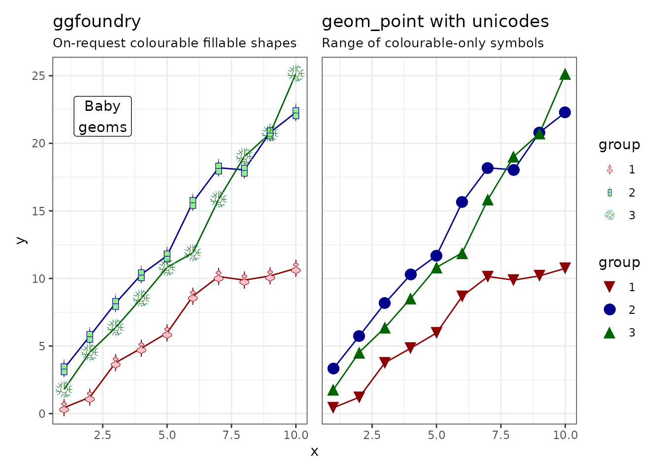
Icons
Icons are also a great option, e.g. for brands. One way to use these as ggplot points is via the showtext and ggtext packages. They too are colourable, but the fill is for the surrounding label rather than the symbol itself. The legend reflects the use of the richtext geom, i.e. shows letters.
library(showtext)
library(ggtext)
font_add("fa-solid", "Font_Awesome_6_Brands-Regular-400.otf")
showtext_auto()
p2 <- p +
geom_richtext(
aes(label = "<span style='font-family: \"fa-solid\"'></span>"),
size = 5, label.colour = NA,
) +
labs(
title = "ggtext with icons",
subtitle = paste0(
"Colourable icons; label fill; ",
"text legend"
)
)
p1 + p2 + plot_layout(guides = "collect", axes = "collect")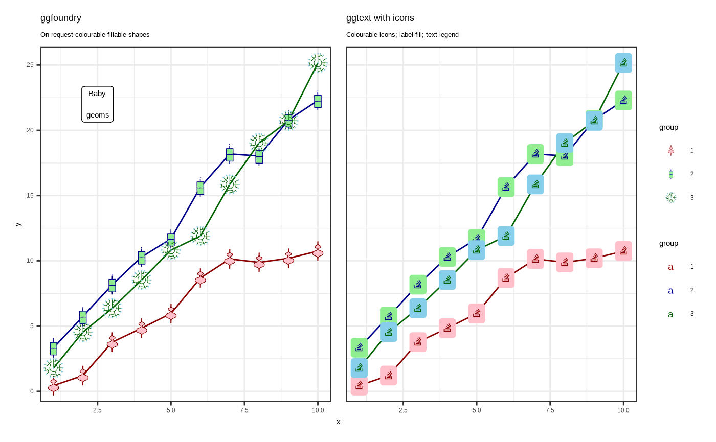
showtext_auto(enable = FALSE)Images
ggimage is a great option for full images, e.g. png files. Country flags, company logos and sports team badges are good example use-cases, as rendering the full image as-is is often the desired outcome.
library(ggimage)

df <- tribble(
  ~x, ~y,
  5, 5,
  6, 6,
  7, 7,
  8, 8
)

p <- df |>
  ggplot(aes(x, y, shape = factor(x), fill = factor(x))) +
  geom_col() +
  scale_fill_viridis_d() +
  scale_y_continuous(limits = c(NA, 9)) +
  theme(plot.subtitle = element_text(size = 10))

p1 <- p +
  geom_casting(size = 0.3, aes(colour = factor(x))) +
  geom_text(aes(label = x, colour = factor(x)), show.legend = FALSE) +
  annotate("label", x = 5.5, y = 8, label = "Polygons") +
  scale_shape_manual(values = c("pentagon", "hexagon", "heptagon", "octagon")) +
  scale_colour_viridis_d(direction = -1) +
  labs(
    title = "ggfoundry",
    subtitle = "Arbitrary hand-crafted fillable shapes"
    )

p2 <- p +
  geom_flag(size = 0.1, image = c("DE", "FR", "CA", "US")) +
  labs(
    title = "ggimage",
    subtitle = "Any as-is whole picture, e.g. png"
    )

p1 + p2 + plot_layout(guides = "collect", axes = "collect")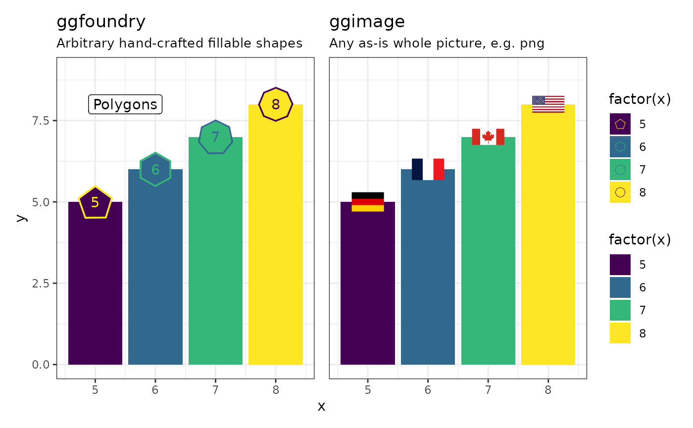
Cunning strategies
Where existing symbols are not fillable, there are possible strategies to achieve a similar effect using only colour and compromising a little on the legend:
- Have one larger layer with a coloured symbol. Then superimpose a smaller second layer with a differently-coloured symbol.
- Use photoshop-style special effects provided by the ggfx package, e.g. adding a differently-coloured outer-glow.
library(ggfx)

df <- tribble(
  ~x, ~y, ~label,
  5, 5, "+",
  6, 6, "x"
)

p <- df |>
  ggplot(aes(x, y, shape = factor(x), fill = factor(x))) +
  geom_col(alpha = 0.5) +
  scale_y_continuous(limits = c(NA, 7)) +
  scale_fill_viridis_d() +
  scale_colour_viridis_d(direction = -1) +
  theme(plot.subtitle = element_text(size = 9))

p1 <- p +
  geom_casting(size = 0.7, aes(colour = factor(x))) +
  geom_text(aes(label = x, colour = factor(x)), show.legend = FALSE) +
  annotate("label", x = 5, y = 6.5, label = "Crosses") +
  scale_shape_manual(values = c("cross2", "cross1")) +
  labs(
    title = "ggfoundry",
    subtitle = "Hand-crafted fillable shapes"
    )

p2 <- p +
  geom_text(aes(label = label), colour = "#22A884", fontface = "bold",
            size = 24, show.legend = FALSE) +
  geom_text(aes(label = label, colour = factor(x)),
            size = 20, show.legend = FALSE) +
  geom_text(aes(label = x), colour = "grey60", nudge_y = -0.15,
            size = 3, show.legend = FALSE) +
  labs(
    title = "Cunning strategy 1",
    subtitle = "Superimposed layers"
    )

p3 <- p +
  with_outer_glow(geom_text(aes(label = label, colour = factor(x)),
    size = 22, show.legend = FALSE,
  ), sigma = 0, expand = 8, colour = "#22A884") +
  geom_text(aes(label = x), colour = "grey60", nudge_y = -0.15,
            size = 3, show.legend = FALSE) +
  labs(
    title = "Cunning strategy 2",
    subtitle = "Photoshop-style outer glow"
  )

p1 + p2 + p3 + plot_layout(guides = "collect", axes = "collect")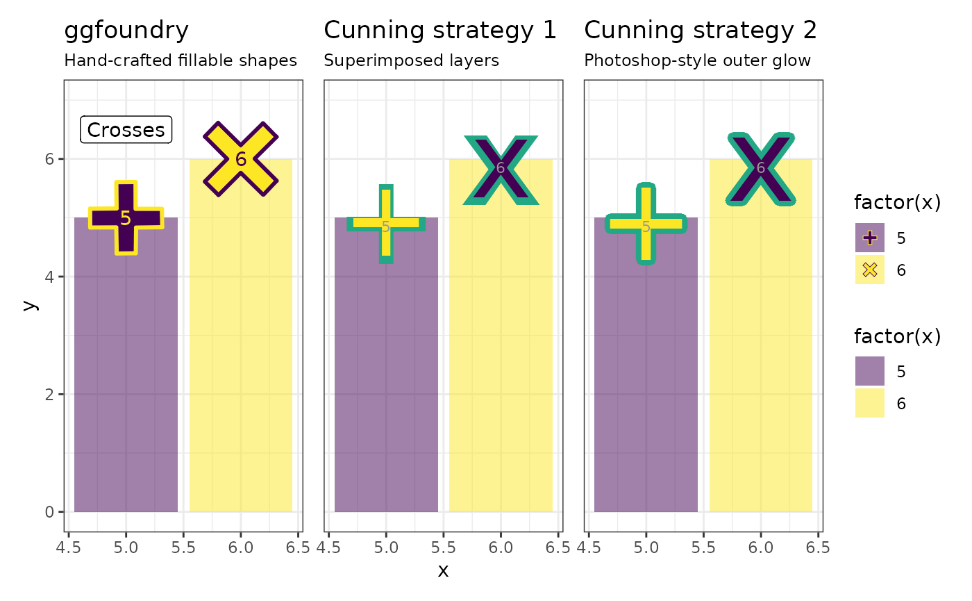
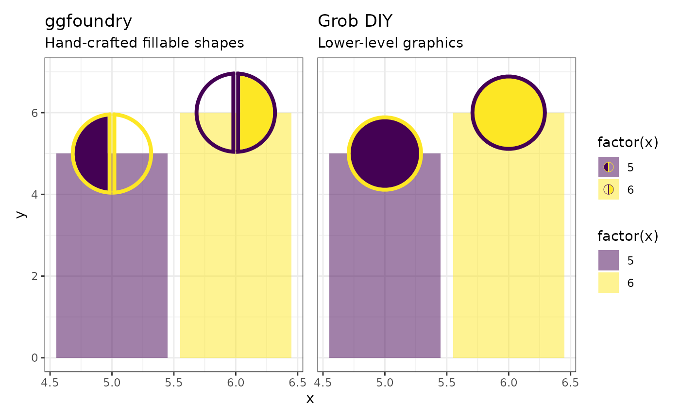
DIY
Making your own grob with grid graphics is a further option. Then use
ggpp and
geom_grob() to add the appropriate layer. A circle is used
here as a very basic example.
library(ggpp)
library(grid)

df <- tibble(
  x = 5:6, y = 5:6,
  grob = c(
    list(circleGrob(r = 0.7, gp = gpar(
      col = "#fde725",
      fill = "#440154",
      lwd = 4
    ))),
    list(circleGrob(r = 0.7, gp = gpar(
      col = "#440154",
      fill = "#fde725",
      lwd = 4
    )))
  )
)

p <- df |>
  ggplot(aes(x, y, shape = factor(x), fill = factor(x))) +
  geom_col(alpha = 0.5) +
  scale_y_continuous(limits = c(NA, 7)) +
  scale_fill_viridis_d() +
  scale_colour_viridis_d(direction = -1)

p1 <- p +
  geom_casting(size = 0.7, aes(colour = factor(x))) +
  annotate("label", x = 5.5, y = 8, label = "Circles") +
  scale_shape_manual(values = c("circleL", "circleR")) +
  labs(
    title = "ggfoundry",
    subtitle = "Hand-crafted fillable shapes"
    )

p2 <- p +
  geom_grob(aes(x, y, label = grob)) +
  labs(
    title = "Grob DIY",
    subtitle = "Lower-level graphics"
  )

p1 + p2 + plot_layout(guides = "collect", axes = "collect")